核密度估计(Kernel Density Estimation, KDE)算法通过样本估计这些样本所属的概率密度函数,是non-parametric方法,也就是在进行估计时无需假设分布的具体形式。本文只讨论单变量(univariate)。
数学表达
给定(n)个样本(x_i in mathcal{R}),通过KDE算法估计(x)处的概率密度为
其中,核函数(K)和带宽(bandwidth)(h)正是KDE算法的两个核心参数。
通过公式(1)易得,如果有(m)个(x)值要估计的概率密度,那么计算时间复杂度是(O(mtimes n))。
Binning
Binning技术是通过将相邻样本分箱到一个box中。分箱之前,我们需要对所有的(n)个样本计算核密度函数值;分箱之后,我们只需要对每个box计算一次即可,然后用它来代表所有被分到这个box内的样本。
根据[1],通过binning计算可分为以下三步:
-
通过将原始数据分配给相邻网格点来对数据进行分箱以获得网格计数。网格计数可以被认为表示其对应网格点附近的数据量。
Bin the data by assigning the raw data to neighboring grid points to obtain grid counts. A grid count can be thought of as representing the amount of data in the neighborhood of its corresponding grid point. -
计算所需的内核权重。网格点等距意味着不同核权重的数量相对较少。
Compute the required kernel weights. The fact that the grid points are equally spaced means that the number of distinct kernel weights is comparatively small. -
结合网格计数和核权重以获得核估计的近似值。这本质上涉及一系列离散卷积。
Combine the grid counts and the kernel weights to obtain the approximation to the kernel estimate. This essentially involves a series of discrete convolutions.
步骤1涉及划分多少个box以及如何将样本对应到box中,对计算速度和精度都非常关键。两种常见的划分方式是
-
Simple Binning: 将样本对应的权重划分到距离到离其最近的grid中。
If a data point at y has surrounding grid points at x and z, then simple binning involves assigning a unit mass to the grid point closest to y. -
Linear Binning: 将样本对应的权重按比例划分到其左右相邻的两个grid中。注意给左端点x和右端点z的权重是和它到两个端点的距离“反过来”的,也就是给x的权重是((z-y)/(z-x)),而给右端点z的权重是((y-x)/(z-x))。
Linear binning assigns a mass of (z - y)/(z - x) to the grid point at x, and (y - x)/(z - x) to the grid point at z.
这里所说的样本权重就是每个样本是否重要性相同,可以联系python代码中sklearn.neighbors.KernelDensity.fit(sample_weight)参数,默认情况下,每个样本地位相同,其权重都为1(或者说都是1/n)。
根据[2],我们可以给Simple Binning一种形式化定义:定义box宽度为(delta)的等距网格(其实也就是对应要划分多少个box),令第(j)个bin的中点表示为(t_j),其包含(n_j)个样本。因此有
不难发现,在上述定义中,内核权重对应为(n_j)(或者说(n_j/nh)),也就是每个box从所有样本中分到的权重是多少。
卷积近似
在binning的第3步中,我们提到结合网格计数和核权重本质上是在做卷积运算,在许多文献中我们也经常可以发现为了加速KDE算法(或解决高维KDE问题)会提到进行卷积近似操作。
首先明确卷积的概念,参考维基百科的定义,卷积是通过两个函数(f)和(g)生成第三个函数的一种数学算子,设(f(t))和(g(t))是实数(mathcal{R})上的两个可积函数,定理两者的卷积为如下特定形式的积分变换:
将公式(3)和公式(4)起来,就不难建立起卷积近似在KDE中的作用了。
Linear Binning + Deriche Approximation
2021年的一篇short paper[3],表明the combination of linear binning and a recursive filter approximation by Deriche可以实现both fast and highly accurate的效果。
Luckily, 作者在Github上公布了开源代码;Unluckily, 代码语言是Javascript;于是我将其翻译为Python版本并公布在Github上。
然而,对于其效果我持怀疑态度,通过运行density1d.py-main,100个高斯分布采样点拟合得到的概率密度函数图像为
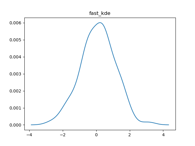

而且,更为关键的问题是无法该代码无法基于样本生成点x处的概率密度?即,在没有人为指定的情况下,代码会默认将[data.min()-pad×bandwidth, data.max()+pad×bandwidth]作为考虑范围,然后将这个区间划分为bins个区间,即((x_0,x_1),(x_1,x_2),...,(x_{text{bins}-1}, x_text{bins})),那么该方法生成的就是(x_0,x_1,...)这些点的概率密度,但如果我希望生成任意一个位置(x, xne x_i)处的概率密度,目前并没有实现。
sklearn.neighbors.KernelDensity
在sklearn库中有KDE算法的实现,而且其考虑采用KD-tree(默认)或Ball-tree来进行加速。
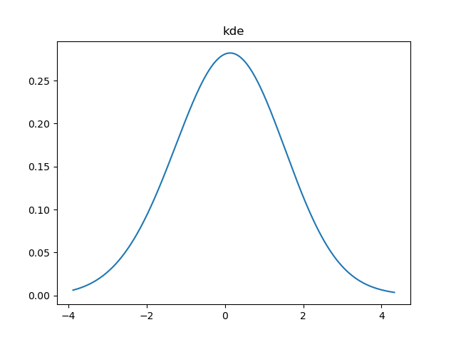
import numpy as np import matplotlib.pyplot as plt from sklearn.neighbors import KernelDensity # 生成一些示例数据 np.random.seed(0) data = np.random.normal(loc=0, scale=1, size=1000) # 创建一个KernelDensity对象 kde = KernelDensity(bandwidth=0.5, kernel='gaussian') # 用示例数据拟合KDE模型 kde.fit(data[:, None]) # 生成一些测试点来评估KDE模型 x = np.linspace(-5, 5, 1000) x = x[:, None] # 使用KDE模型评估密度 log_density = kde.score_samples(x) # 绘制原始数据和KDE估计的密度曲线 plt.figure(figsize=(10, 6)) plt.hist(data, bins=30, density=True, alpha=0.5, color='blue') plt.plot(x, np.exp(log_density), color='red', lw=2) plt.title('Kernel Density Estimation (KDE)') plt.xlabel('Value') plt.ylabel('Density') plt.show() 这是非常简单的一个例子,简单到甚至我之前没有思考为什么要先kde.fit()才能评估密度kde.score_sample()。通过公式(1),我们可以发现只要清楚指定的核函数(K)和带宽(bandwidth)(h),那么就可以计算出任意一点的概率密度,而这两个参数都是在创建KDE对象时就指定好的。
起初,我以为kde.fit()是在训练参数(h),甚至有那么一瞬间让我觉得困扰我们如何指定超参数(h)的值根本不是问题,因为它只是个初始值,而在fit之后会训练到最好的参数。这种思路明显是错的。因为缺乏ground_truth,因此模型本身就缺乏训练(h)的能力,这也是为什么(h)被称作超参数更合适而非参数。
既然核函数和带宽都是指定好的,那么如果我们不fit直接去评估密度呢?
import numpy as np from sklearn.neighbors import KernelDensity # 生成一些示例数据 np.random.seed(0) data = np.random.normal(loc=0, scale=1, size=1000) # 创建一个KernelDensity对象 kde = KernelDensity(bandwidth=0.5, kernel='gaussian') # 生成一些测试点来评估KDE模型 x = np.linspace(-5, 5, 1000) x = x[:, None] # 使用KDE模型评估密度 log_density = kde.score_samples(x) Traceback (most recent call last): File "D:pythonfast_kdemain.py", line 17, in <module> log_density = kde.score_samples(x) ^^^^^^^^^^^^^^^^^^^^ File "F:anaconda3Libsite-packagessklearnneighbors_kde.py", line 261, in score_samples check_is_fitted(self) File "F:anaconda3Libsite-packagessklearnutilsvalidation.py", line 1462, in check_is_fitted raise NotFittedError(msg % {"name": type(estimator).__name__}) sklearn.exceptions.NotFittedError: This KernelDensity instance is not fitted yet. Call 'fit' with appropriate arguments before using this estimator. 看起来,sklearn要求在调用kde.score_samples()必须要kde.fit()。
通过阅读源代码,kde.fit()没有改变任何KDE的参数,但构建了内置对象self.tree_,这个就是我们前面提到的KD-tree或Ball-tree,而在进行评估时也是基于这个tree进行的。我的理解是,KD-tree维护样本之间的距离信息,在评估一个新的数据(x)处的概率密度时,和它距离太远的样本就不计算了?
References
[1] @article{wand1994fast,
title = {Fast Computation of Multivariate Kernel Estimators},
author = {Wand, M. P.},
year = {1994},
journal = {Journal of Computational and Graphical Statistics},
volume = {3},
number = {4},
pages = {433},
doi = {10.2307/1390904}
}
[2] @article{wand1994fast,
title = {Fast Computation of Multivariate Kernel Estimators},
author = {Wand, M. P.},
year = {1994},
journal = {Journal of Computational and Graphical Statistics},
volume = {3},
number = {4},
pages = {433},
doi = {10.2307/1390904}
}
[3] @inproceedings{heer2021fast,
title = {Fast & Accurate Gaussian Kernel Density Estimation},
booktitle = {2021 IEEE Visualization Conference (VIS)},
author = {Heer, Jeffrey},
year = {2021},
pages = {11--15},
publisher = {IEEE},
address = {New Orleans, LA, USA},
doi = {10.1109/VIS49827.2021.9623323},
isbn = {978-1-66543-335-8},
langid = {english}
}