
模拟退火算法(Simulated Annealing, SA)是一种受物理中固体退火过程启发的元启发式优化算法,用于在大规模搜索空间中寻找近似全局最优解。其核心思想是通过模拟物理退火过程中的“温度”下降和粒子热运动,逐步收敛到低能量(即目标函数更优)的状态。
一、基本原理
1. 物理退火类比
在固体退火中,材料被加热至高温后缓慢冷却,原子从高能态逐渐趋于有序排列,最终达到能量最低的稳定状态。模拟退火算法将这一过程抽象为:
温度(T):控制搜索的随机性。
能量(E):对应目标函数值(需最小化的代价或最大化的问题的适应度)。
2. Metropolis准则
算法以一定概率接受比当前解更差的解,避免陷入局部最优。
对于新解(x_{new})和当前解(x_{current}):
若(Delta E=E(x_{mew})-E(x_{current})leq 0 quad (更优解)),直接接受。
若(Delta E > 0 quad (更差解)),以概率(P=e^{-Delta E/T})接受。
3. 温度调度(Cooling Schedule)
初始高温时,算法广泛探索解空间;随着温度降低,逐渐倾向于局部优化。
温度下降方式:如指数下降(T_{k+1}=alpha T_k quad (alphain(0,1)为冷却系数))。
二、算法步骤
1. 初始化
随机生成初始解(x_0)。
设置初始温度(T_0) 、终止温度(T_{min})、冷却系数(alpha)。
2. 迭代过程
生成新解:在当前解附近随机扰动(如交换、位移等操作)产生候选解(x_{new})。
评估解:计算目标函数差值(Delta E)。
接受准则:根据Metropolis准则决定是否接受(x_{new})。
降温:更新温度(T=alpha T)。
终止条件:温度降至(T_{min}) 或达到最大迭代次数。
三、参数选择
初始温度:足够高以使初始接受概率接近1(如(P_{initial}approx 0.8))。
冷却系数:典型值(alpha in [0.85,0.99])。
终止条件:温度趋近于0或解长时间无改进。
四、算法特点及优缺点
算法特点
逃离局部最优:通过概率性接受劣解,增强全局搜索能力。
收敛性:在足够慢的降温速度下,理论上能以概率1收敛到全局最优解(但实际中难以实现)。
灵活性:适用于连续或离散优化问题,只需定义解表示、邻域结构和目标函数。
优缺点
优点:简单通用,适合非线性、多峰问题。
缺点:收敛速度慢,参数调优依赖经验。
五、应用场景
组合优化(如旅行商问题TSP、调度问题)。
函数优化(连续/非凸函数)。
机器学习(参数调优、神经网络训练)。
六、Python实现示例
import matplotlib matplotlib.use('TkAgg') import numpy as np import matplotlib.pyplot as plt plt.rcParams['font.sans-serif'] = ['SimHei'] # 中文支持 plt.rcParams['axes.unicode_minus'] = False # 负号显示 # 目标函数:Rastrigin函数,常用于优化算法测试 def objective_function(x): A = 10 # Rastrigin函数参数 n = len(x) # 问题维度 return A * n + sum([(xi ** 2 - A * np.cos(2 * np.pi * xi)) for xi in x]) # 模拟退火算法实现 def simulated_annealing(initial_state, objective_function, initial_temperature=100, cooling_rate=0.95, num_iterations=1000, perturbation_scale=0.1): # 初始化当前状态和最优状态 current_state = initial_state.copy() best_state = initial_state.copy() current_energy = objective_function(current_state) best_energy = current_energy # 记录迭代过程 energies = [current_energy] temperatures = [initial_temperature] states = [current_state.copy()] temperature = initial_temperature for iteration in range(num_iterations): # 生成邻域解(扰动当前解) neighbor = current_state + np.random.normal(0, perturbation_scale, len(current_state)) # 计算新解的能量 neighbor_energy = objective_function(neighbor) # 计算能量差 delta_energy = neighbor_energy - current_energy # 判断是否接受新解 if delta_energy < 0 or np.random.rand() < np.exp(-delta_energy / temperature): current_state = neighbor current_energy = neighbor_energy # 更新最优解 if current_energy < best_energy: best_state = current_state.copy() best_energy = current_energy # 降温 temperature *= cooling_rate # 记录当前迭代结果 energies.append(current_energy) temperatures.append(temperature) states.append(current_state.copy()) # 打印进度 if (iteration + 1) % 100 == 0: print(f"Iteration {iteration + 1}/{num_iterations}, " f"Current Energy: {current_energy:.4f}, " f"Best Energy: {best_energy:.4f}, " f"Temperature: {temperature:.4f}") return { 'best_state': best_state, 'best_energy': best_energy, 'energies': np.array(energies), 'temperatures': np.array(temperatures), 'states': np.array(states) } # 运行模拟退火算法 np.random.seed(42) # 设置随机种子以便结果可重现 initial_state = np.random.uniform(-5.12, 5.12, 2) # 二维Rastrigin函数的初始解 result = simulated_annealing( initial_state, objective_function, initial_temperature=100, cooling_rate=0.99, num_iterations=2000, perturbation_scale=0.5 ) # 打印结果 print("n优化结果:") print(f"最优解: {result['best_state']}") print(f"最优值: {result['best_energy']:.4f}") # 可视化优化过程 plt.figure(figsize=(15, 5)) # 绘制能量变化曲线 plt.subplot(1, 2, 1) plt.plot(result['energies']) plt.title('能量变化') plt.xlabel('迭代次数') plt.ylabel('能量值') plt.grid(True) # 绘制温度变化曲线 plt.subplot(1, 2, 2) plt.plot(result['temperatures']) plt.title('温度变化') plt.xlabel('迭代次数') plt.ylabel('温度') plt.grid(True) plt.tight_layout() plt.show() 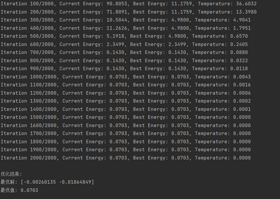
示例实现了模拟退火算法来求解 Rastrigin 函数的最小值。代码包含以下部分:
目标函数:定义了 Rastrigin 函数作为优化目标
算法实现:完整的模拟退火算法,包括解的扰动、接受准则和温度更新
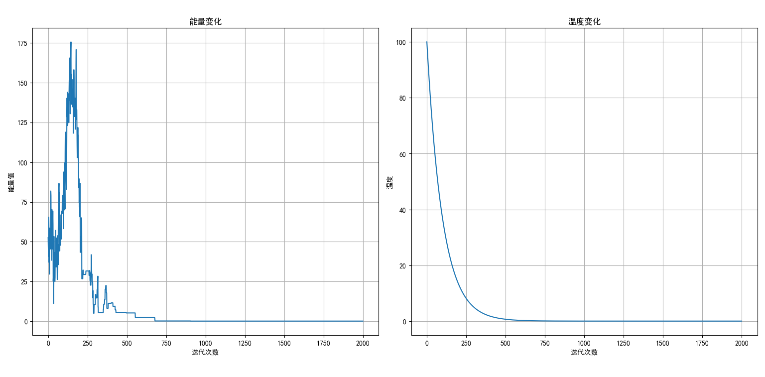
可视化:展示优化过程中能量和温度的变化趋势
主要参数包括初始温度、降温速率、迭代次数和扰动规模,可根据需要调整这些参数来优化搜索效果。
七、小结
模拟退火算法通过 “高温探索、低温收敛” 的策略,平衡了随机性(跳出局部最优)和确定性(向全局最优收敛),是一种高效的全局优化方法。


![洛谷 P11345 [KTSC 2023 R2] 基地简化 题解](http://www.itfaba.com/wp-content/themes/kemi/timthumb.php?src=http://www.itfaba.com/wp-content/themes/kemi/img/random/1.jpg&w=218&h=124&zc=1)
