
逻辑回归介绍

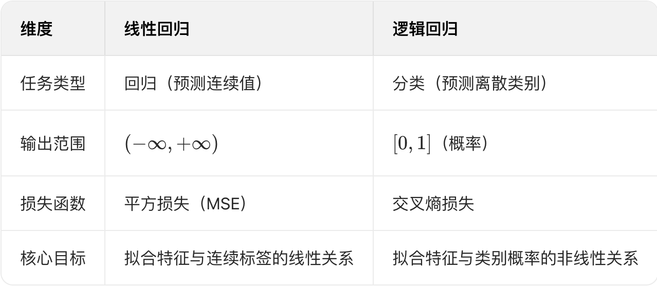
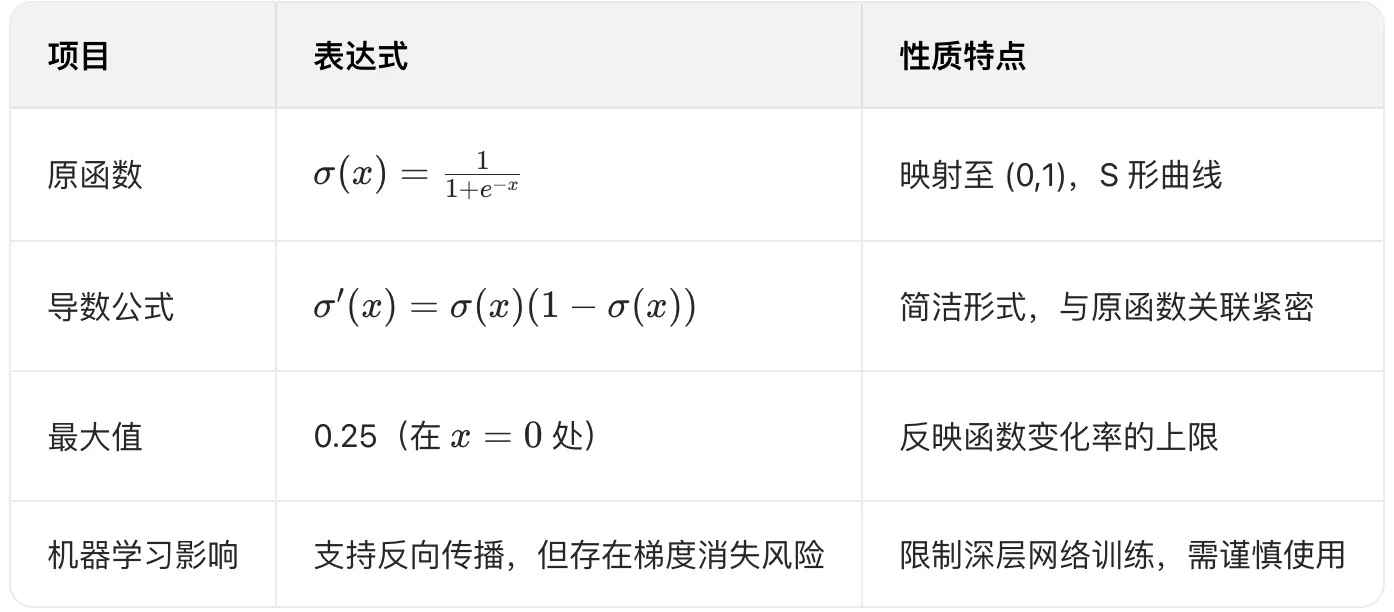
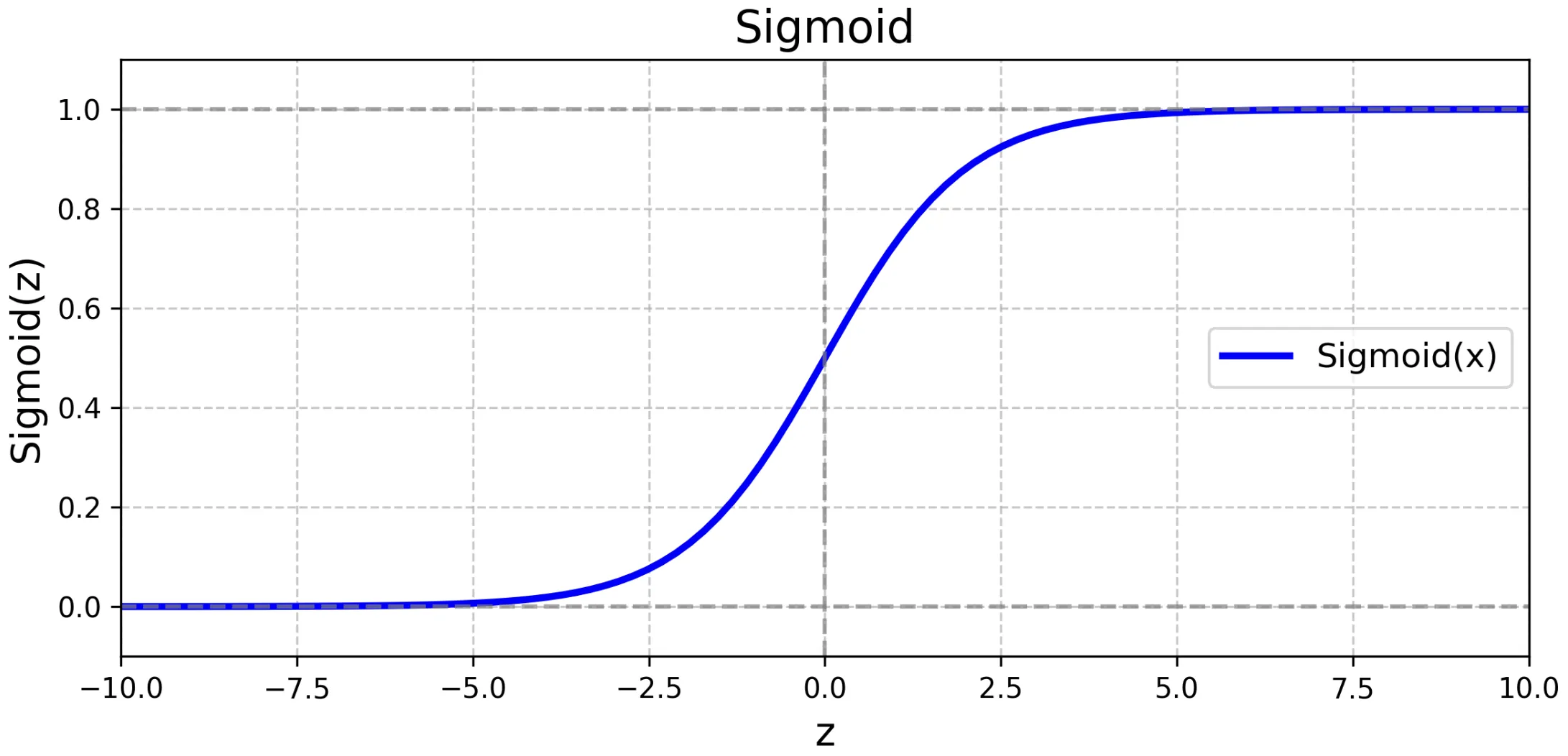
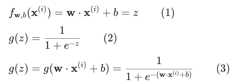
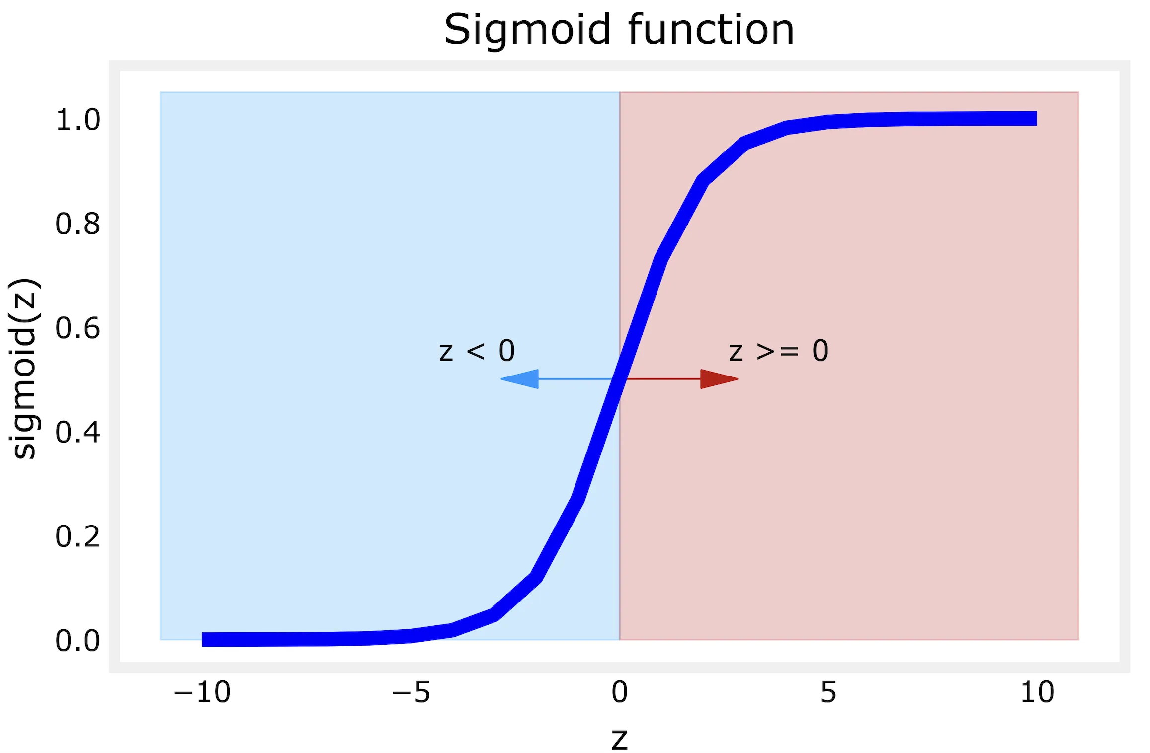
sigmoid函数
def sigmoid(z): """ Compute the sigmoid of z Args: z (ndarray): A scalar, numpy array of any size. Returns: g (ndarray): sigmoid(z), with the same shape as z """ g = 1 / (1 + np.exp(-z)) return g
逻辑回归模型
逻辑回归的决策边界
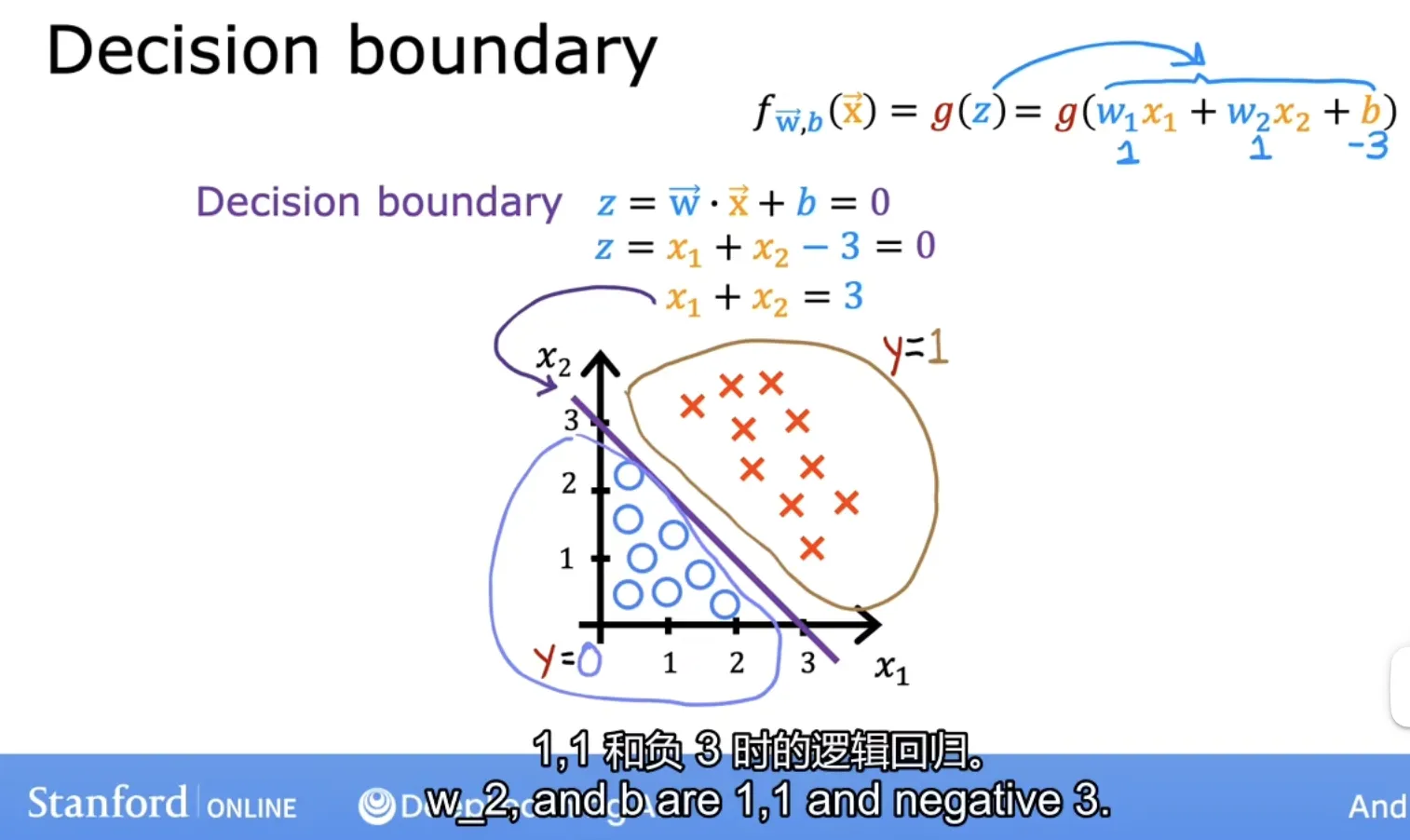
线性逻辑回归
根据sigmoid函数图象:z=0是中间位置,视为决策边界;那么为了得到决策边界的特征情况,我们假设:
- 线性模型
z = w1 * x1 + w2 * x2 + b - 参数
w1=w2=1, b=03,那么x2 = -x1 + 3这条直线就是决策边界
如果特征x在这条线的右边,那么此逻辑回归则预测为1,反之则预测为0;(分为两类)
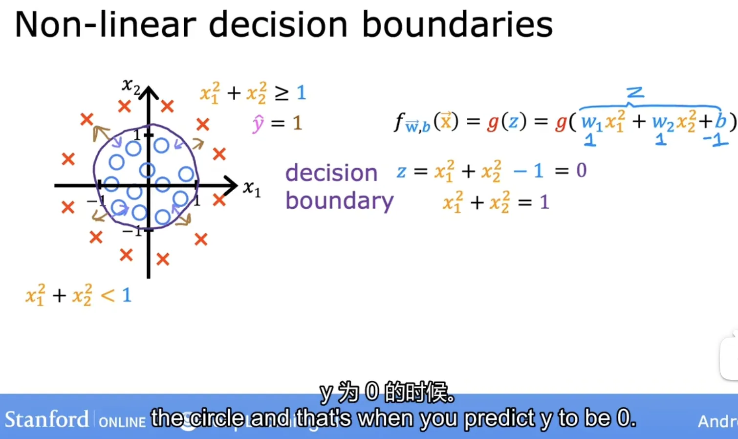
多项式逻辑回归
多项式回归决策边界,我们假设:
- 多项式模型:
z = w1 * x1**2 + w2 * x2**2 + b - 参数:
w1=w2=1, b=-1
如果特征x在圆的外面,那么此逻辑回归则预测为1,反之则预测为0;(分为两类)
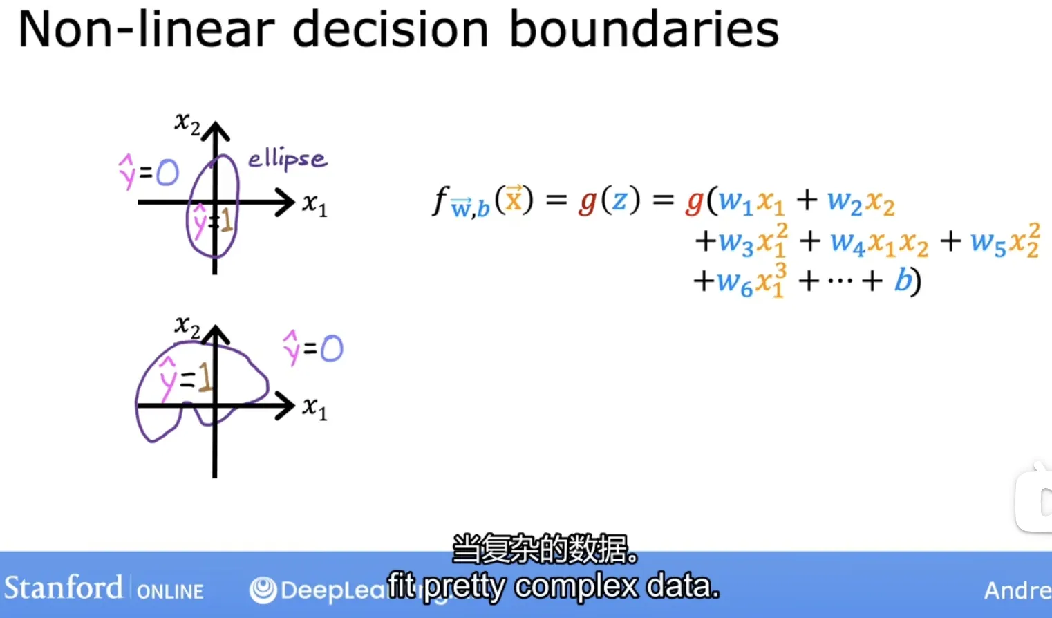
扩展:随着多项式的复杂度增加,还可以拟合更更多非线性的复杂情况
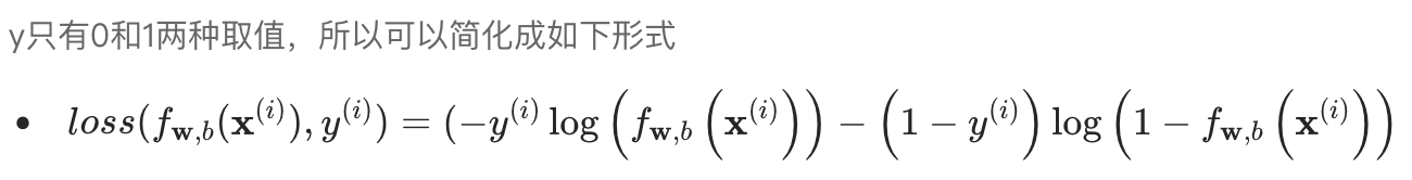
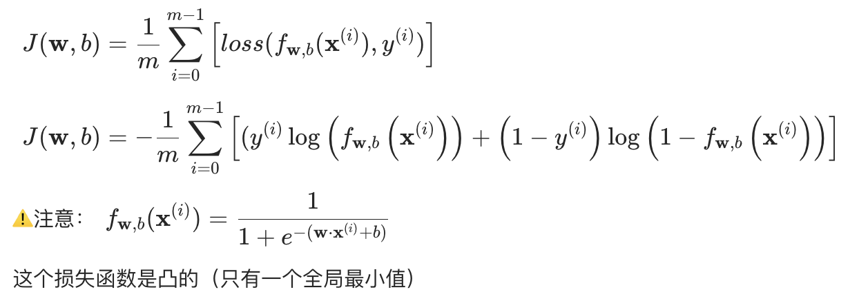
逻辑回归的损失函数
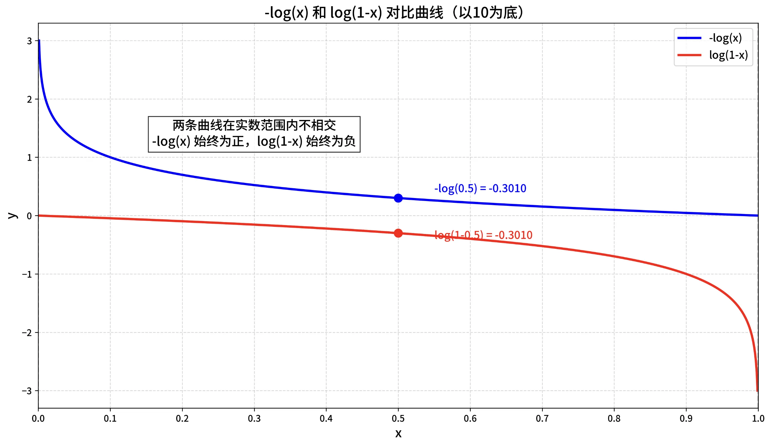
平方损失和交叉熵损失
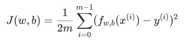
回顾下线性回归的损失函数(平方损失):
平方误差损失函数不适用于逻辑回归模型:平方损失在逻辑回归中是 “非凸函数”(存在多个局部最优解),难以优化;
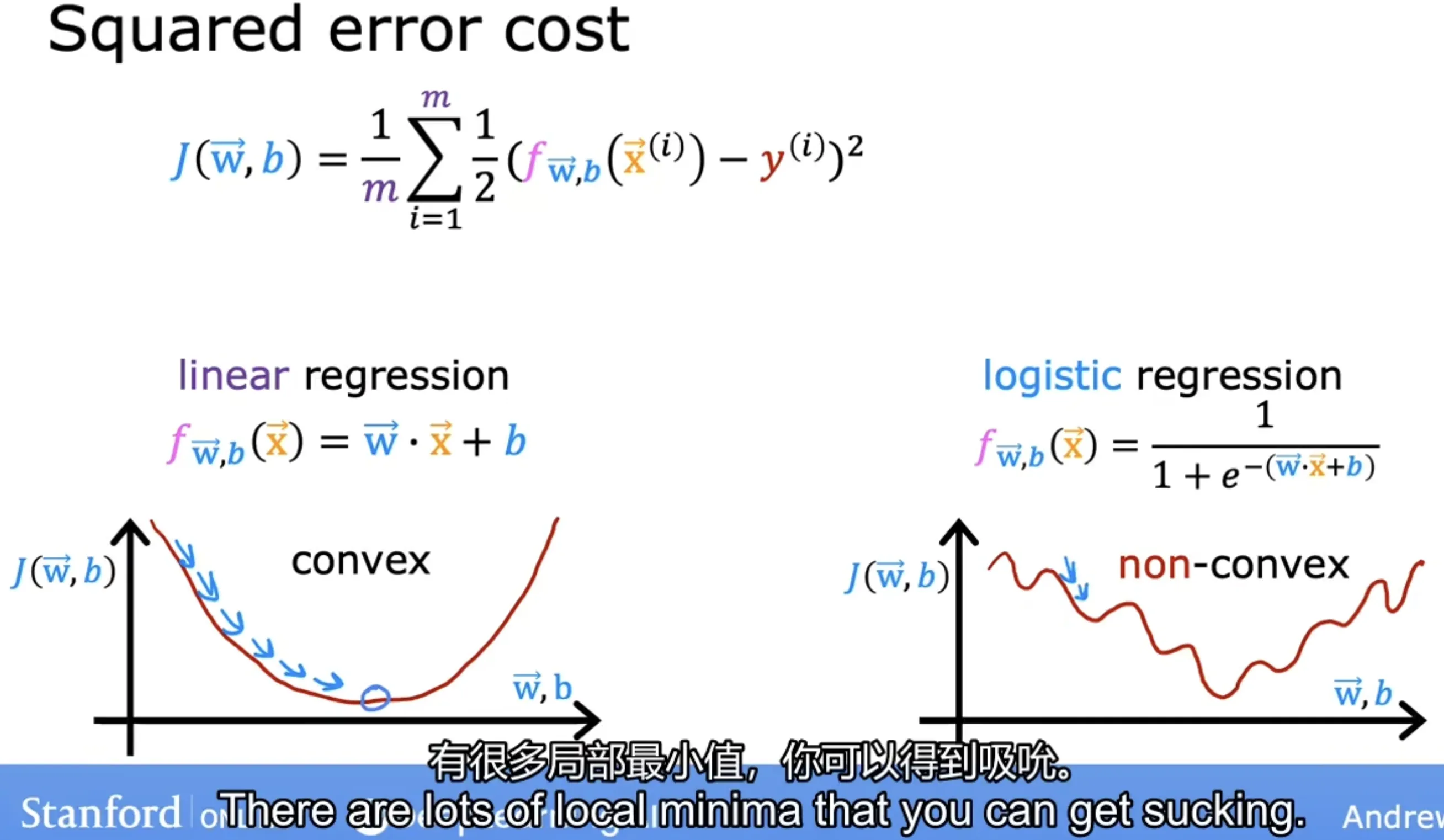
所以我们需要一个新的损失函数,即交叉熵损失;交叉熵损失是 “凸函数”,可通过梯度下降高效找到全局最优。
交叉熵源于信息论,我们暂时不做深入介绍,直接给出交叉熵损失函数公式:
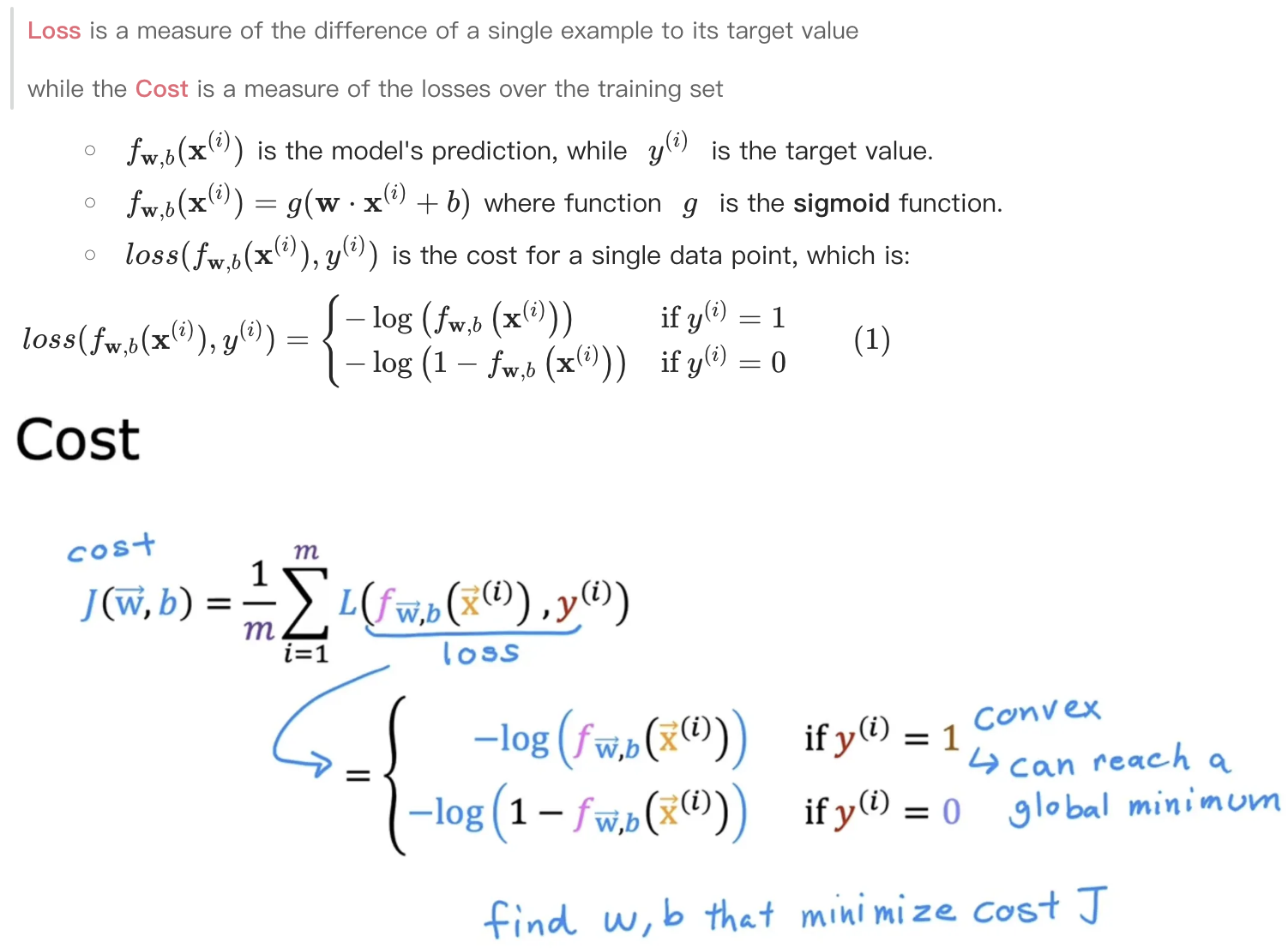
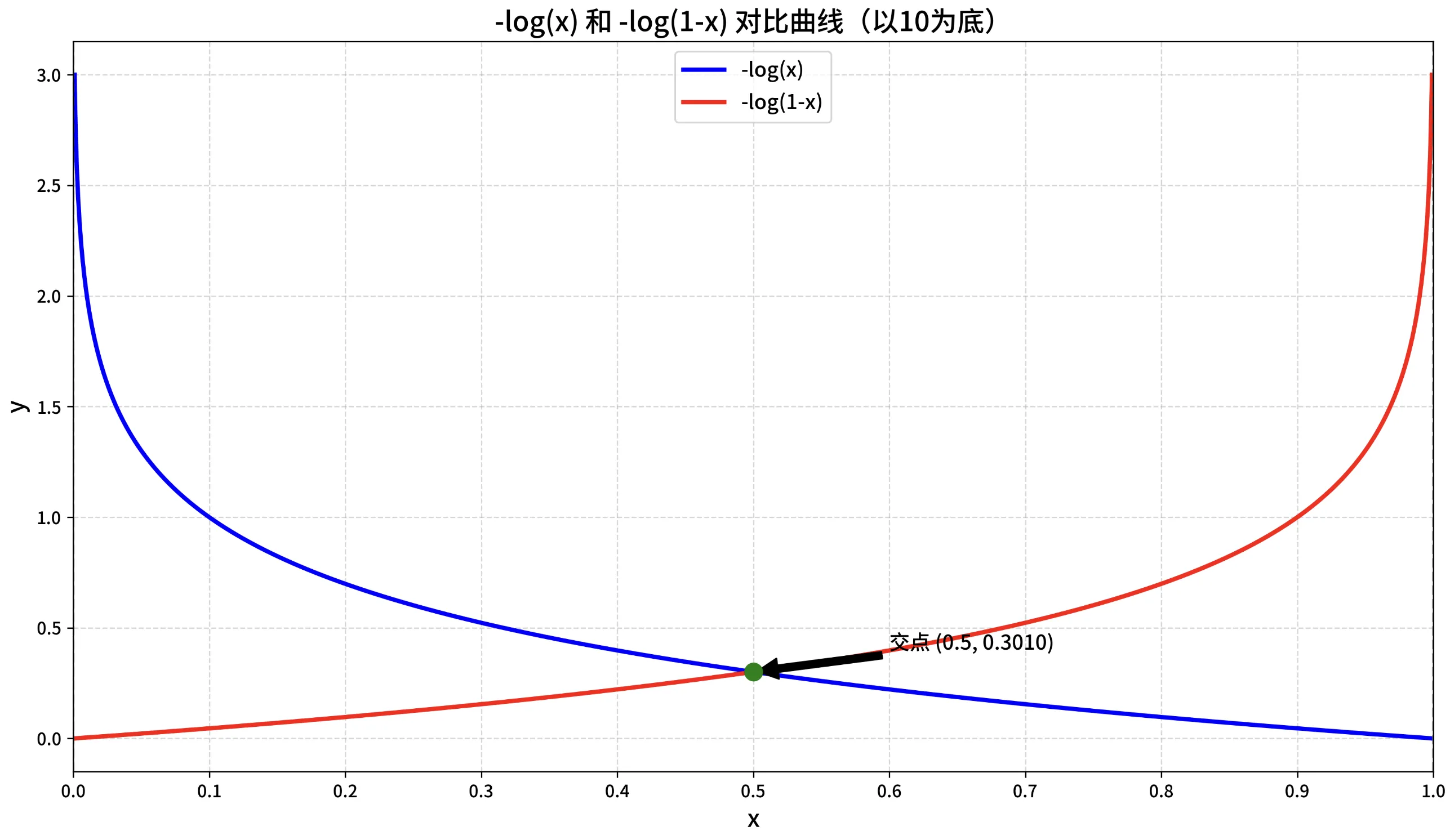
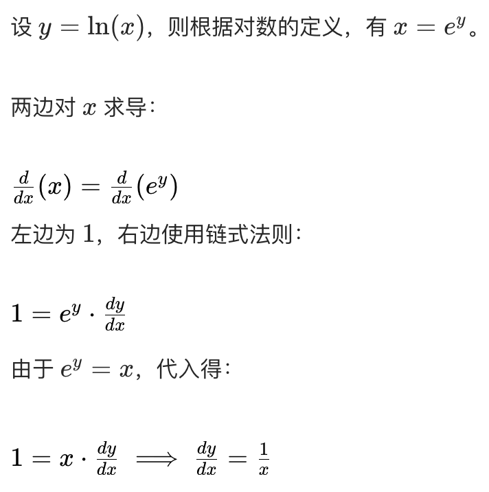
对数回顾
复习下对数函数的性质,以便理解为什么 交叉熵损失是 “凸函数”?
简化交叉熵损失函数
为什么要用这个函数来表示?来源自 最大释然估计(Maximum Likelihood),这里不做过多介绍。
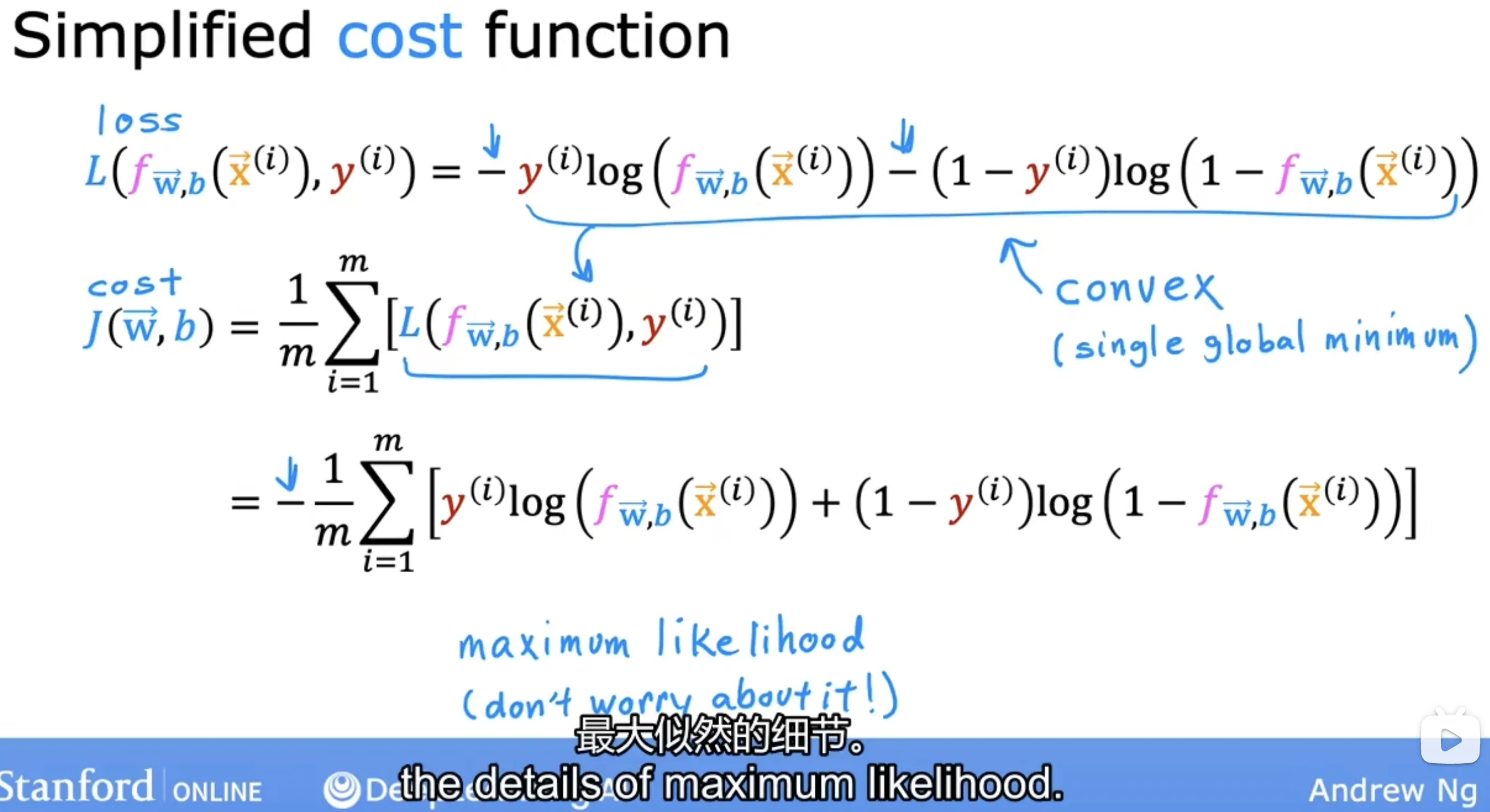
简化结果:
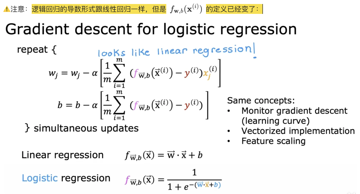
逻辑回归的梯度计算
自然对数求导公式:
链式求导法则:
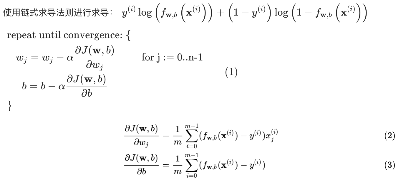
⚠️注意:
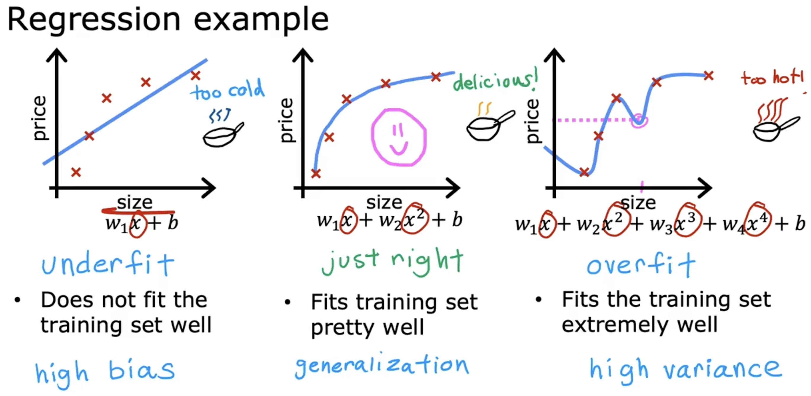
过拟合问题
线性回归过拟合
逻辑回归过拟合
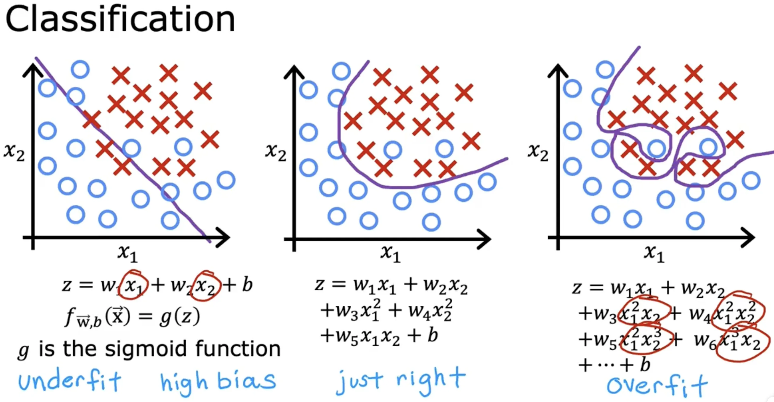
- 欠拟合(underfit),存在高偏差(bias)
- 泛化(generalization):希望我们的学习算法在训练集之外的数据上也能表现良好(预测准确)
- 过拟合(overfit),存在高方差(variance)
解决过拟合的办法
- 特征选择:只选择部分最相关的特征(基于直觉intuition)进行训练;缺点是丢掉了部分可能有用的信息
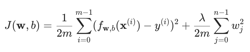
- 正则化:正则化是一种更温和的减少某些特征的影响,而无需做像测地消除它那样苛刻的事:
- 鼓励学习算法缩小参数,而不是直接将参数设置为0(保留所有特征的同时避免让部分特征产生过大的影响)
- 鼓励把 w1 ~ wn 变小,b不用变小
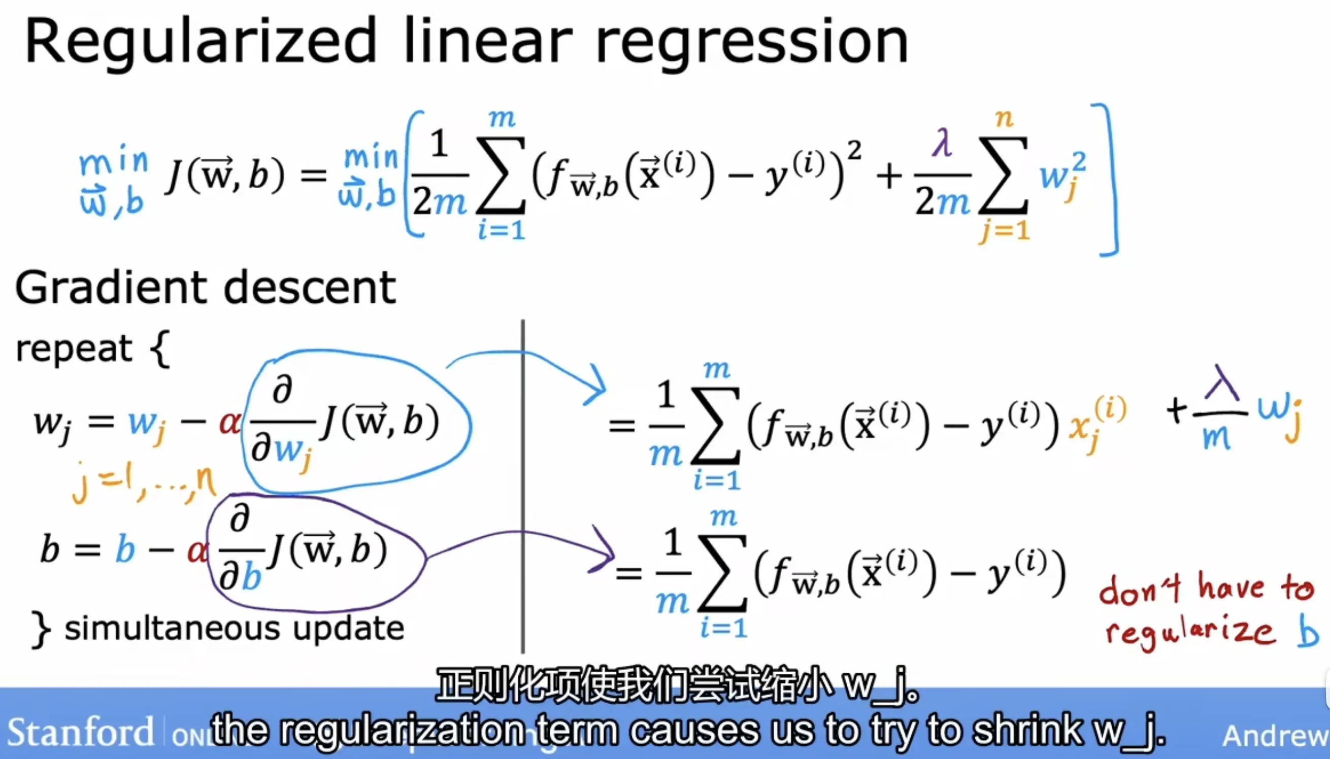
正则化模型
It turns out that regularization is a way
to more gently reduce ths impacts of some of the features without doing something as harsh as eliminating it outright.
关于正则化项的说明:
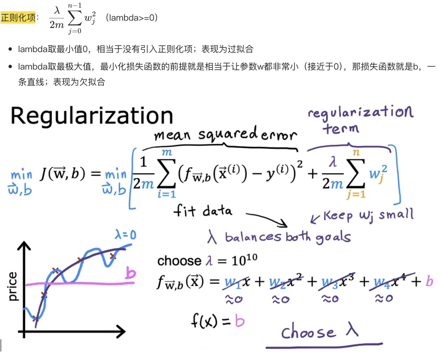
带正则化项的损失函数
正则化线性回归
损失函数:
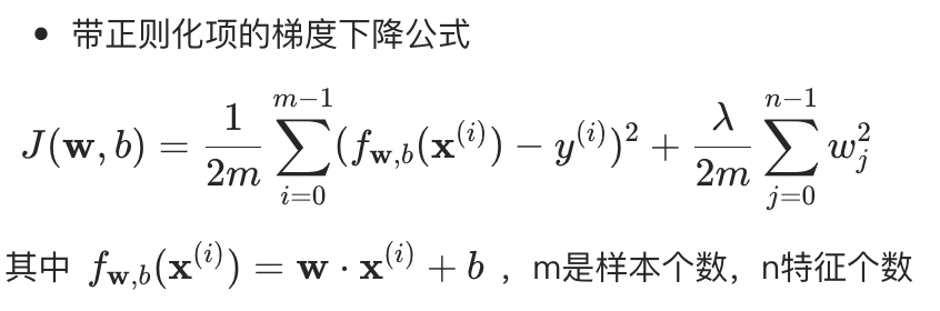
梯度计算:
分析梯度计算公式,由于alpha和lambda通常是很小的值,所以相当于在每次迭代之前把参数w缩小了一点点,这也就是正则化的工作原理,如下所示:

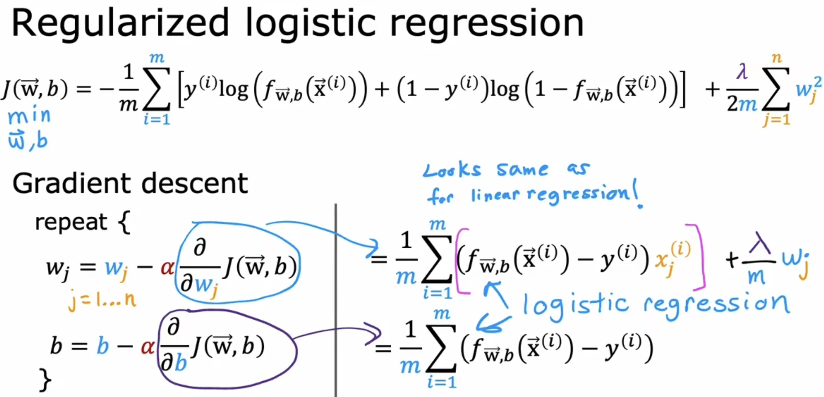
正则化逻辑回归
损失函数:
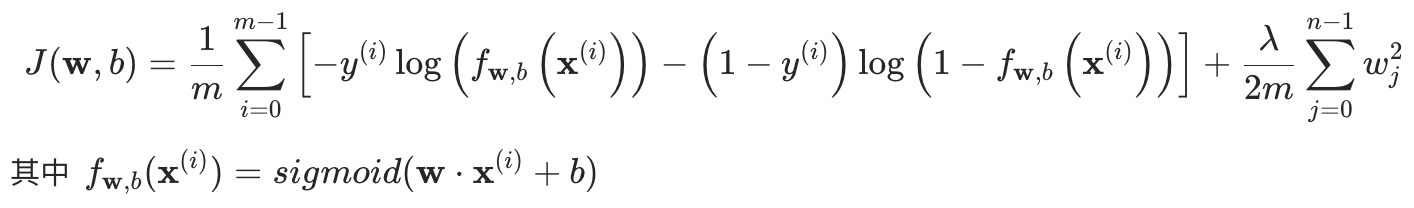
梯度计算:
线性回归和逻辑回归正则化总结
逻辑回归实战
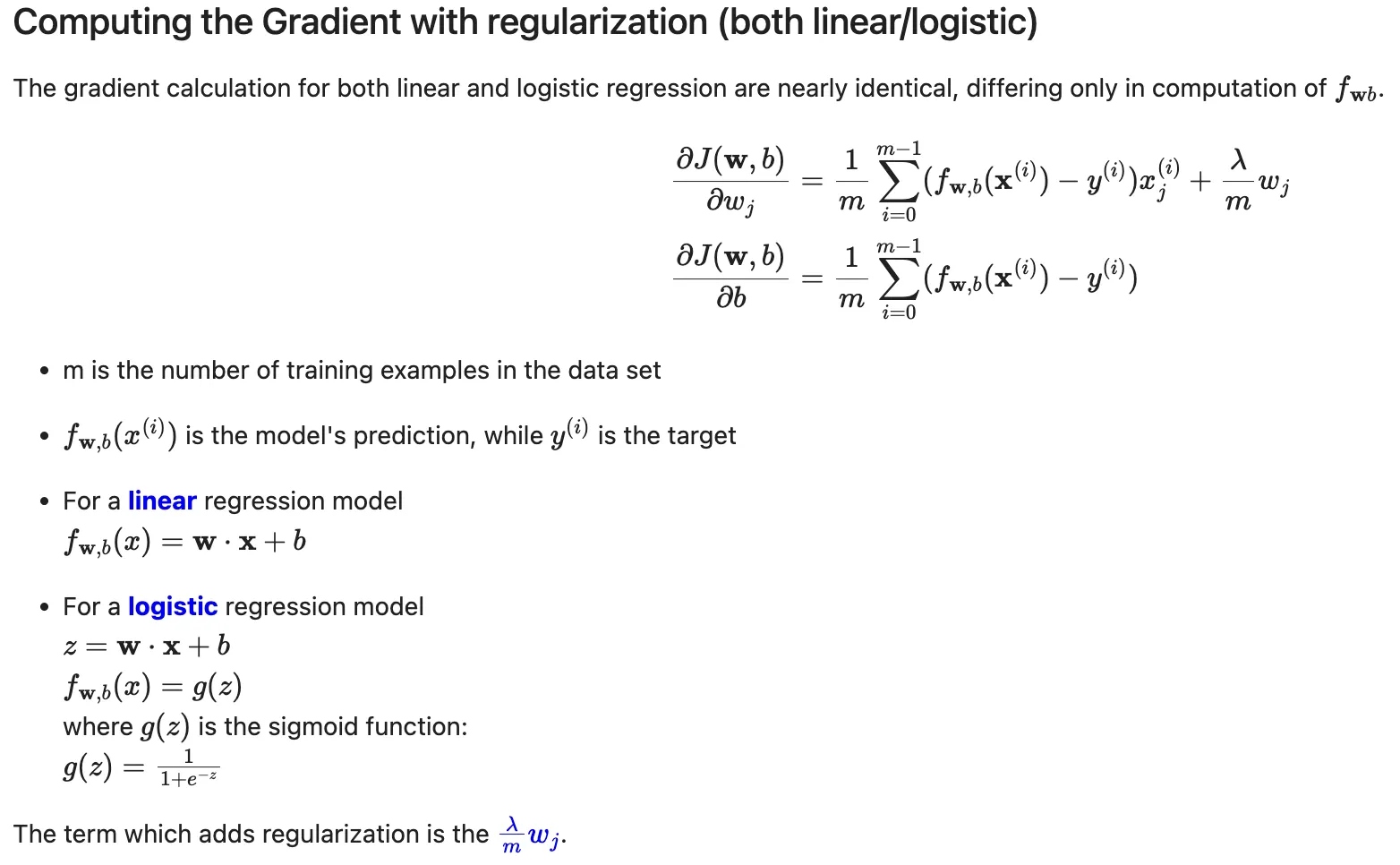
模型选择
可视化训练数据,基于此数据选择线性逻辑回归模型
关键代码实现
def sigmoid(z): g = 1 / (1 + np.exp(-z)) return g def compute_cost(X, y, w, b, lambda_= 1): """ Computes the cost over all examples Args: X : (ndarray Shape (m,n)) data, m examples by n features y : (array_like Shape (m,)) target value w : (array_like Shape (n,)) Values of parameters of the model b : scalar Values of bias parameter of the model lambda_: unused placeholder Returns: total_cost: (scalar) cost """ m, n = X.shape total_cost = 0 for i in range(m): f_wb_i = sigmoid(np.dot(X[i], w) + b) loss = -y[i] * np.log(f_wb_i) - (1 - y[i]) * np.log(1 - f_wb_i) total_cost += loss total_cost = total_cost / m return total_cost def compute_gradient(X, y, w, b, lambda_=None): """ Computes the gradient for logistic regression Args: X : (ndarray Shape (m,n)) variable such as house size y : (array_like Shape (m,1)) actual value w : (array_like Shape (n,1)) values of parameters of the model b : (scalar) value of parameter of the model lambda_: unused placeholder. Returns dj_dw: (array_like Shape (n,1)) The gradient of the cost w.r.t. the parameters w. dj_db: (scalar) The gradient of the cost w.r.t. the parameter b. """ m, n = X.shape dj_dw = np.zeros(n) dj_db = 0. for i in range(m): f_wb_i = sigmoid(np.dot(X[i], w) + b) diff = f_wb_i - y[i] dj_db += diff for j in range(n): dj_dw[j] = dj_dw[j] + diff * X[i][j] dj_db = dj_db / m dj_dw = dj_dw / m return dj_db, dj_dw def gradient_descent(X, y, w_in, b_in, cost_function, gradient_function, alpha, num_iters, lambda_): """ Performs batch gradient descent to learn theta. Updates theta by taking num_iters gradient steps with learning rate alpha Args: X : (array_like Shape (m, n) y : (array_like Shape (m,)) w_in : (array_like Shape (n,)) Initial values of parameters of the model b_in : (scalar) Initial value of parameter of the model cost_function: function to compute cost alpha : (float) Learning rate num_iters : (int) number of iterations to run gradient descent lambda_ (scalar, float) regularization constant Returns: w : (array_like Shape (n,)) Updated values of parameters of the model after running gradient descent b : (scalar) Updated value of parameter of the model after running gradient descent """ # number of training examples m = len(X) # An array to store cost J and w's at each iteration primarily for graphing later J_history = [] w_history = [] w = copy.deepcopy(w_in) b = b_in for i in range(num_iters): dj_db, dj_dw = gradient_function(X, y, w, b, lambda_) w = w - alpha * dj_dw b = b - alpha * dj_db cost = cost_function(X, y, w, b, lambda_) J_history.append(cost) w_history.append(w) if i % math.ceil(num_iters / 10) == 0: print(f"{i:4d} cost: {cost:6f}, w: {w}, b: {b}") return w, b, J_history, w_history #return w and J,w history for graphing def predict(X, w, b): m, n = X.shape p = np.zeros(m) for i in range(m): f_wb = sigmoid(np.dot(X[i], w) + b) p[i] = f_wb >= 0.5 return p
结果展示
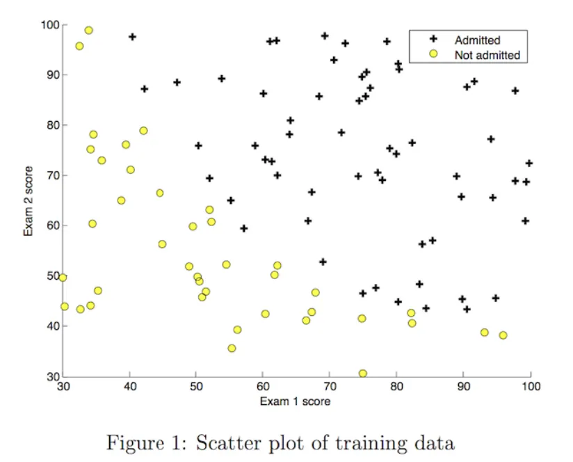
import numpy as np import matplotlib.pyplot as plt import matplotlib.font_manager as fm # 支持显示中文 font_path = '/System/Library/Fonts/STHeiti Light.ttc' custom_font = fm.FontProperties(fname=font_path) plt.rcParams["font.family"] = custom_font.get_name() # 载入训练集 X_train, y_train = load_data("data/ex2data1.txt") # 训练模型 np.random.seed(1) intial_w = 0.01 * (np.random.rand(2).reshape(-1,1) - 0.5) initial_b = -8 iterations = 10000 alpha = 0.001 w_out, b_out, J_history,_ = gradient_descent(X_train ,y_train, initial_w, initial_b, compute_cost, compute_gradient, alpha, iterations, 0) # 根据训练结果(w_out和b_out)计算决策边界 #f = w0*x0 + w1*x1 + b # x1 = -1 * (w0*x0 + b) / w1 plot_x = np.array([min(X_train[:, 0]), max(X_train[:, 0])]) plot_y = (-1. / w_out[1]) * (w_out[0] * plot_x + b_out) # 将训练数据分类 x0s_pos = [] x1s_pos = [] x0s_neg = [] x1s_neg = [] for i in range(len(X_train)): x = X_train[i] # print(x) y_i = y_train[i] if y_i == 1: x0s_pos.append(x[0]) x1s_pos.append(x[1]) else: x0s_neg.append(x[0]) x1s_neg.append(x[1]) # 绘图 plt.figure(figsize=(8, 6)) plt.scatter(x0s_pos, x1s_pos, marker='o', c='green', label="Admitted") plt.scatter(x0s_neg, x1s_neg, marker='x', c='red', label="Not admitted") plt.plot(plot_x, plot_y, lw=1, label="决策边界") plt.xlabel('Exam 1 score', fontsize=12) plt.ylabel('Exam 2 score', fontsize=12) plt.title('在二维平面上可视化分类模型的决策边界', fontsize=14) plt.legend(fontsize=12, loc='upper center') plt.grid(True) plt.show() # 使用训练集计算预测准确率 p = predict(X_train, w_out, b_out) print('Train Accuracy: %f'%(np.mean(p == y_train) * 100)) # Train Accuracy: 92.000000
正则化逻辑回归实战
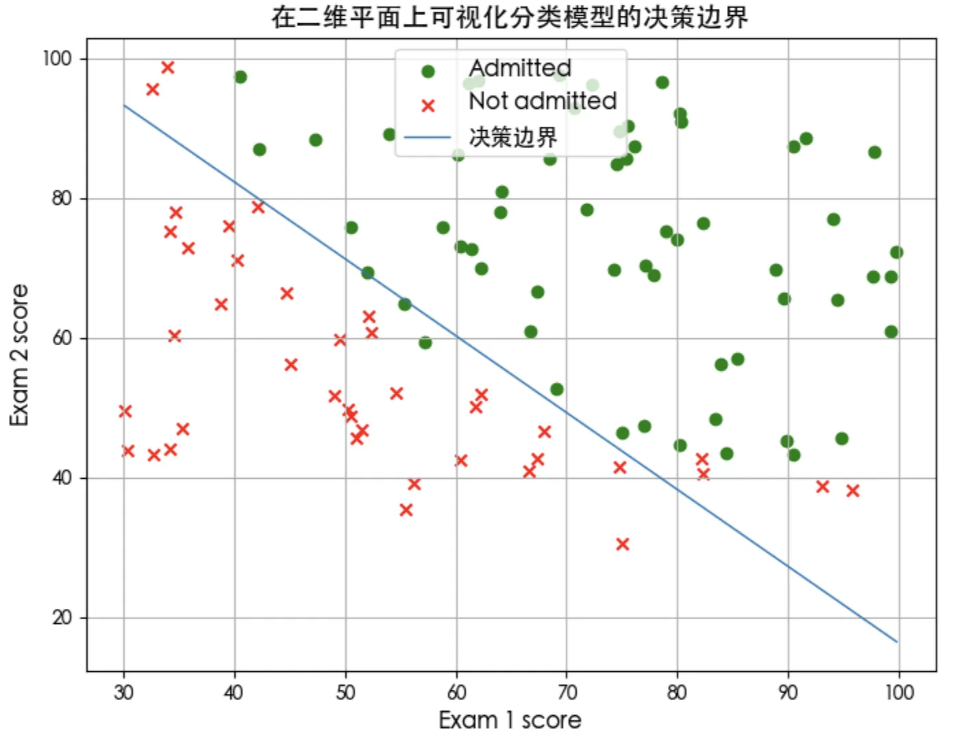
模型选择
可视化训练数据,基于此数据选择多项式逻辑回归模型
关键代码实现
由于要拟合非线性决策边界,所以要增加特征的复杂度(训练数据里只有2个特征)。
特征映射函数
# 将输入特征 X1 和 X2 转换为六次多项式特征 # 这个函数常用于逻辑回归或支持向量机等模型中,通过增加特征的复杂度来拟合非线性决策边界。 def map_feature(X1, X2): """ Feature mapping function to polynomial features """ X1 = np.atleast_1d(X1) X2 = np.atleast_1d(X2) degree = 6 out = [] for i in range(1, degree+1): for j in range(i + 1): out.append((X1**(i-j) * (X2**j))) return np.stack(out, axis=1)
正则化后的损失函数和梯度计算函数
def compute_cost_reg(X, y, w, b, lambda_ = 1): """ Computes the cost over all examples Args: X : (array_like Shape (m,n)) data, m examples by n features y : (array_like Shape (m,)) target value w : (array_like Shape (n,)) Values of parameters of the model b : (array_like Shape (n,)) Values of bias parameter of the model lambda_ : (scalar, float) Controls amount of regularization Returns: total_cost: (scalar) cost """ m, n = X.shape # Calls the compute_cost function that you implemented above cost_without_reg = compute_cost(X, y, w, b) reg_cost = 0. for j in range(n): reg_cost += w[j]**2 # Add the regularization cost to get the total cost total_cost = cost_without_reg + (lambda_/(2 * m)) * reg_cost return total_cost def compute_gradient_reg(X, y, w, b, lambda_ = 1): """ Computes the gradient for linear regression Args: X : (ndarray Shape (m,n)) variable such as house size y : (ndarray Shape (m,)) actual value w : (ndarray Shape (n,)) values of parameters of the model b : (scalar) value of parameter of the model lambda_ : (scalar,float) regularization constant Returns dj_db: (scalar) The gradient of the cost w.r.t. the parameter b. dj_dw: (ndarray Shape (n,)) The gradient of the cost w.r.t. the parameters w. """ m, n = X.shape dj_db, dj_dw = compute_gradient(X, y, w, b) # Add the regularization for j in range(n): dj_dw[j] += (lambda_ / m) * w[j] return dj_db, dj_dw
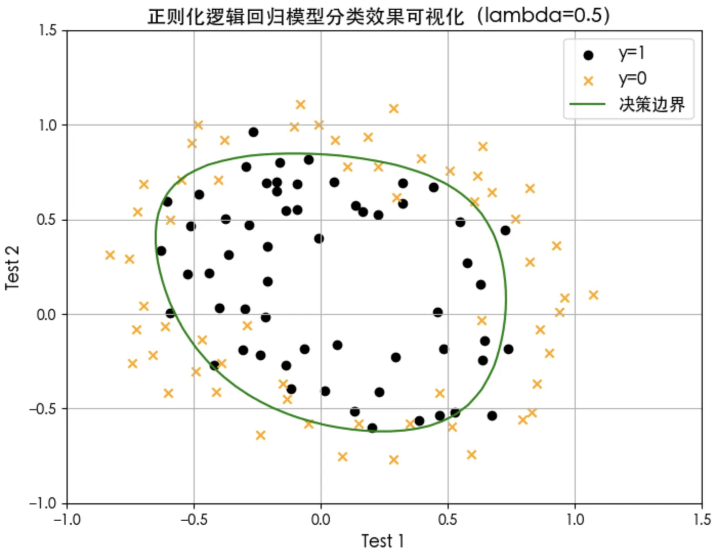
结果展示
import numpy as np import matplotlib.pyplot as plt import matplotlib.font_manager as fm # 支持显示中文 font_path = '/System/Library/Fonts/STHeiti Light.ttc' custom_font = fm.FontProperties(fname=font_path) plt.rcParams["font.family"] = custom_font.get_name() # 载入训练集 X_train, y_train = load_data("data/ex2data2.txt") # 通过增加特征的复杂度来拟合非线性决策边界 X_mapped = map_feature(X_train[:, 0], X_train[:, 1]) print("Original shape of data:", X_train.shape) print("Shape after feature mapping:", X_mapped.shape) # 训练模型 np.random.seed(1) initial_w = np.random.rand(X_mapped.shape[1])-0.5 initial_b = 1. # Set regularization parameter lambda_ to 1 (you can try varying this) lambda_ = 0.5 iterations = 10000 alpha = 0.01 w_out, b_out, J_history, _ = gradient_descent(X_mapped, y_train, initial_w, initial_b, compute_cost_reg, compute_gradient_reg, alpha, iterations, lambda_) # 根据训练结果(w_out和b_out)计算决策边界 # - 创建网格点 u 和 v 覆盖特征空间 u = np.linspace(-1, 1.5, 50) v = np.linspace(-1, 1.5, 50) # - 计算每个网格点处的预测概率 z z = np.zeros((len(u), len(v))) # Evaluate z = theta*x over the grid for i in range(len(u)): for j in range(len(v)): z[i,j] = sig(np.dot(map_feature(u[i], v[j]), w_out) + b_out) # - 转置 z 是必要的,因为contour函数期望的输入格式与我们的计算顺序不一致 z = z.T # 分类 x0s_pos = [] x1s_pos = [] x0s_neg = [] x1s_neg = [] for i in range(len(X_train)): x = X_train[i] # print(x) y_i = y_train[i] if y_i == 1: x0s_pos.append(x[0]) x1s_pos.append(x[1]) else: x0s_neg.append(x[0]) x1s_neg.append(x[1]) # 绘图 plt.figure(figsize=(8, 6)) plt.scatter(x0s_pos, x1s_pos, marker='o', c='black', label="y=1") plt.scatter(x0s_neg, x1s_neg, marker='x', c='orange', label="y=0") # 绘制决策边界(等高线) plt.contour(u,v,z, levels = [0.5], colors="green") # 创建虚拟线条用于图例(颜色和线型需与等高线一致) plt.plot([], [], color='green', label="决策边界") plt.xlabel('Test 1', fontsize=12) plt.ylabel('Test 2', fontsize=12) plt.title('正则化逻辑回归模型分类效果可视化(lambda=0.5)', fontsize=14) # plt.legend(fontsize=12, loc='upper center') plt.legend(fontsize=12) plt.grid(True) plt.show() #Compute accuracy on the training set p = predict(X_mapped, w_out, b_out) print('Train Accuracy: %f'%(np.mean(p == y_train) * 100)) # Train Accuracy: 83.050847
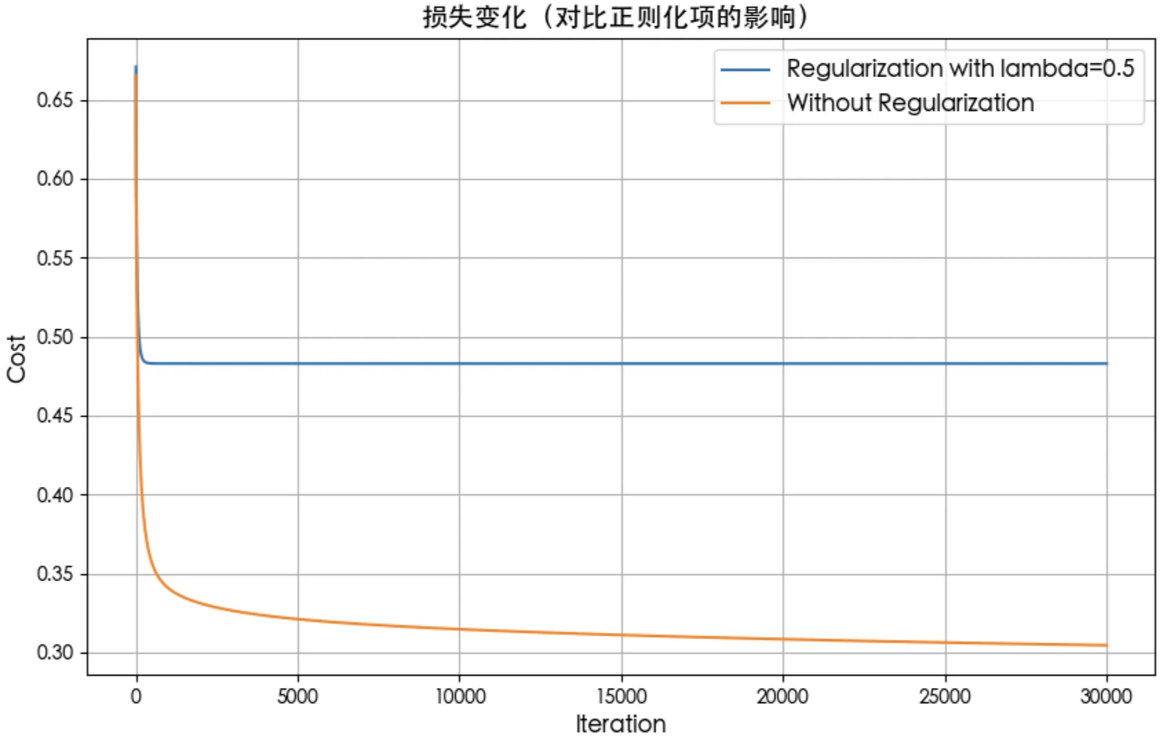
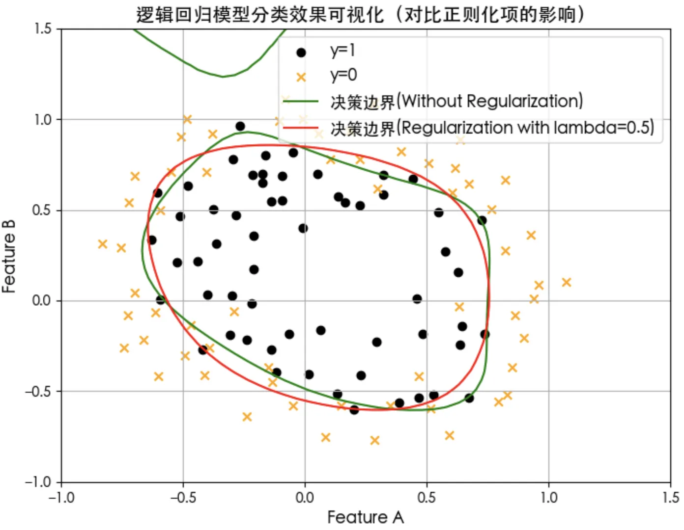
正则化效果对比
正则化对损失和决策边界的影响
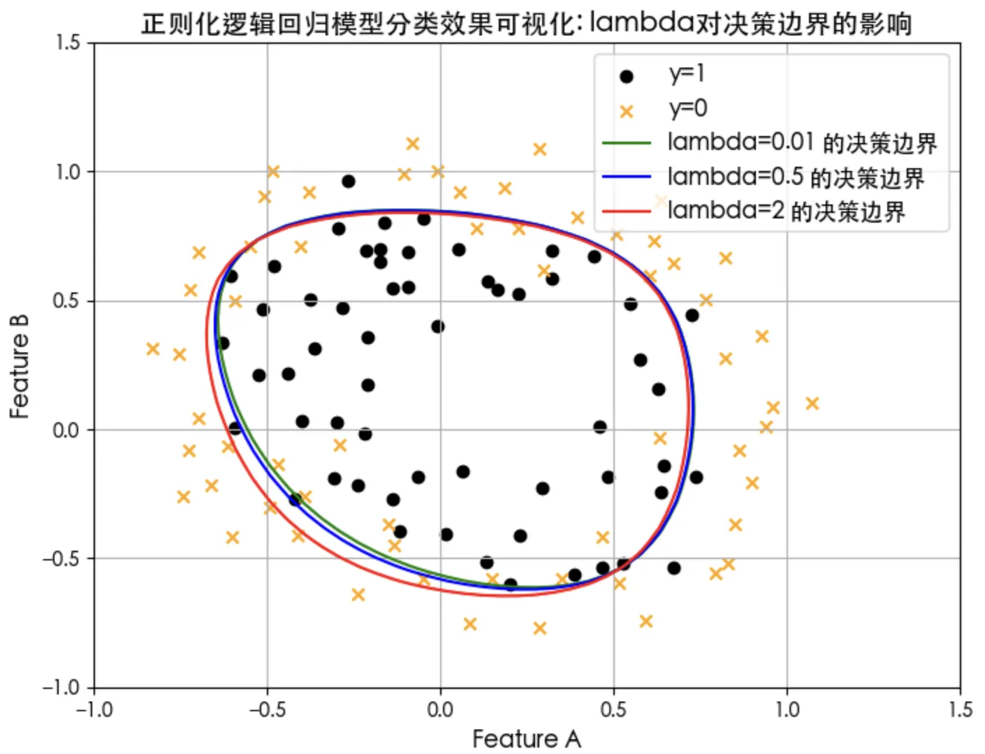
正则化项lambda参数大小对决策边界的影响
参考
吴恩达团队在Coursera开设的机器学习课程:https://www.coursera.org/specializations/machine-learning-introduction
在B站学习:https://www.bilibili.com/video/BV1Pa411X76s


![洛谷 P11345 [KTSC 2023 R2] 基地简化 题解](http://www.itfaba.com/wp-content/themes/kemi/timthumb.php?src=http://www.itfaba.com/wp-content/themes/kemi/img/random/1.jpg&w=218&h=124&zc=1)
